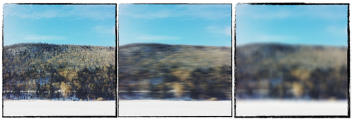
Image convolution for blurring should have been a simple concept to implement, but it’s been hard for me to wrap my head around how to perform convolution on a 2D (and 3-tuple) set of pixels, and how that works algorithmically, so this is a bit of a brain dump to help me sort out how it actually works.

Naïve Box Blur

My first blur implementation was a quick-and-dirty (colloquially known as the naïve) method of box blur. Box blur is a simple average of all the neighboring pixels surrounding one, so it’s a uniformly weighted blur algorithm. The naïve implementation looks something like this:

for each row
    for each col
        set count to 0
        for every neighboring pixel within the radius m in the x direction
            for every neighboring pixel within the radius m in the y direction
                 add the color to the total
                 count++
        final_color = total/count
        setpixel(current x, current y, final_color)

This algorithm is O(n^2 * m^2). It is very slow when running a 10px blur on a 500x500px image, which is a pretty standard request on an honestly less-than-standard picture resolution. Thankfully, this can be improved.

Better Box Blur

The first step for speed is to split up the inner nested for loops for calculating the average color at a pixel. Turns out, if you blur in one dimension, then take the result and blur in the other dimension, you get the same output as if you were to blur both dimensions simultaneously. Also, this has the added benefit of giving you some nice code to abstract into standalone 1D motion blurs should you need them later. The pseudocode now looks like this

for each row
    for each col
        set count to 0
        for every neighboring pixel within the radius m in the x direction
             add the color to the total
             count++
        final_color = total/count
        setpixel(current x, current y, final_color)

repeat above for y direction

This gets us down from O(n^2 * m^2) to O(n^2 * 2m), and feels markedly faster in execution.

Even Better Box Blur

If we’re clever though, this can be made even faster. I always understood convolution best through visualizing the moving average filter. Since box blur is effectively a 2D moving average filter, this is a great place to start.

The box blur takes a moving average at every pixel.

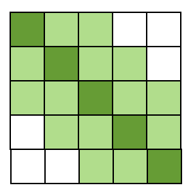
But if you examine what happens at consecutive steps, a better intuition for the moving average is that you subtract one element from the left side and add one element from the right side to your “total color” value, and then average. Since it moves element-by-element, a lot of values are repeated. Rather than starting from scratch for each pixel’s average, we can just take the previous pixels’ average, subtract the leftmost pixel from the prior average, and add one more on the right side. The algorithm looks like this now:

for each row
    // get the window for the first pixel
    for every neighboring pixel within the radius m in the x direction
        add the color to the total
        count++
    final_color = total/count
    setpixel(0, current y, final_color)

    //now we use the window for the 0th pixel
    for (pixel 1 in zero, pixel < width; pixel++)
           total -= color(pixel - blursize)
           total += color(pixel + blursize)
           final_color = total/(2*blursize + 1)
           setpixel(current x, current y, final_color)

repeat above for the columns

This pseudocode doesn’t appropriately handle edge cases, such as if you’re close to an edge and your average is less than (2 * blursize + 1). If you don’t account for this you’ll have vignetting around the edge of your image, which can be aesthetic but for this disucssion looks novice.

That’s it! From here it’s easy to apply weights to have the pixel average adhere to a normal distribution a la Gauss, and just use negative weights for an easy sharpening filter.